Recap

In the last section we discussed the difference between an analytical and a numerical solution. We finished with an example of how to calculate the first three steps of a numerical method to solve the 3D equations of motion of a projectile. There is one last piece we haven't discussed yet, and that is how to get the reference drag coefficient Cdref.

Getting the Cdref value - Linear Interpolation

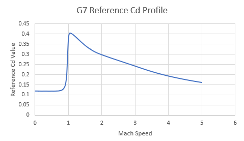
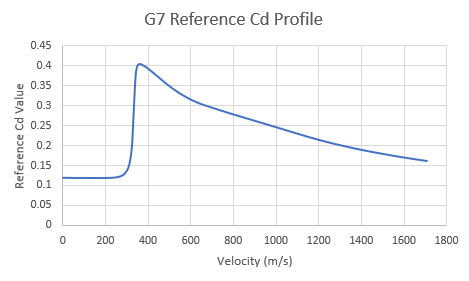
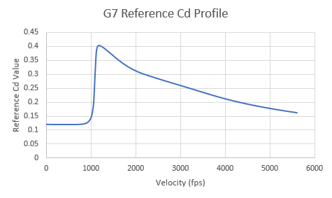
In the above example, we glossed over the explanation of how to get the Cdref value. Recall these previous charts, the Cdref value changes with the velocity of the projectile:

G7 Profile: Cdref vs Mach speed

G7 Profile: Cdref vs Velocity (m/s) @ ICAO Conditions: 15 deg C, speed of sound (c)= 340.3 m/s

G7 Profile: Cdref vs Velocity (ft/s) @ ICAO Conditions: 59 deg F, speed of sound (c) = 1116.5 fps

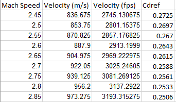
The table used to generate these graphs looks like this:

If we look back to our example above, the velocity at t=0 was 900 m/s. If you look at the above table, you can see there is an entry for 888 m/s and 905 m/s. So how do we get the Cdref value for 900 m/s? Linear interpolation is a mathematical technique for this precise situation, it lets us approximate the correct value between two entries in a table.

Intuitively, it is quite easy to understand how the technique works. Given the example above, 900 m/s is in between 888 m/s and 905 m/s. What is the midpoint between 888 and 905?

We start by taking the difference of 905 and 888:

Divide this by two:

Then add back the smaller number (888):

The midpoint between the two numbers is 896.5.

Now let’s assume that the value for Cdref changes in a straight line over this small interval. We can find the Cdref at the midpoint:

• Cdref @ 905 = 0.2615
• Cdref @ 888 = 0.2643

• Cdref @ 896.5 = 0.2629

Since we know that 900 is in between 896.5 and 905, we also know that the Cdref @ 900 will be in between 0.2629 and 0.2615.

Linear interpolation works along this same principle. However, instead of taking the halfway point, it calculates exactly how far the value is in between the two outer values.

Imagine you have a number line:

The difference between 900 and 888 is 12.

The difference between 905 and 888 is 17.

If we take a ratio of these numbers, we can see that 900 is 0.71 or 71% of the way between 888 and 905.

Now we need to find the corresponding Cdref value that is 71% of the way in between 0.2643 and 0.2615.

We can work in reverse using simple algebra (x is a placeholder variable):

Now instead of doing this math piece by piece, we can summarize it all into one equation:

• v: velocity for which we want Cdref

• v1: velocity of lower bound

• v2: velocity of upper bound

• Cdref: Cdref we are solving for

• Cdref1: Cdref @ v1

• Cdref2: Cdref @ v2

Since the ratio is the same across both equations, we can set them equal to each other:

Now we need to rearrange the equation to get Cdref:

If you are a visual learner, here is an illustration of the process:

Lets double check we get the same answer:

That is the essence of linear interpolation, and with this technique we can get a value for Cdref at any velocity as long as there is a value above and below it in the table.

IMPORTANT: This technique only works when the distance between data points is small. For example, if you tried to linearly interpolate the Cdref @ 500m/s between the velocities of 100 m/s and 1000 m/s, you will not get an accurate result. Linear interpolation works on the assumption that the data between two points would fall on a straight line if you connected them. In the case of our table above, the velocities are roughly 20m/s apart which is sufficiently accurate for our purposes.

Next article: Calculating Trajectory: Installation and Configuration of Python and VSCode